Tensors

Below are two statements to be considered:

(One) When a basis for a vector is transformed using a direct transformation, the inverse of that transformation transforms the coordinates of the vector.

(Two) A basis for an n-dimensional vector space V is any ordered set of linearly independent vectors $(e_1, e_2, e_3, ..., e_n)$ . With these basis vectors it is possible to express any vector ‘x’ with coordinates $(x^1, x^2, x^3, ..., x^n)$ .

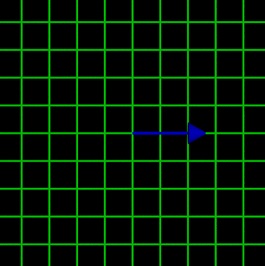
Imagine that you’ve drawn a vector that has a length of 1 inch and it points to the right (or if you prefer, to the east). You declare arrows pointing to the right as being positive.

Here’s were it gets a little bit difficult. Please play along–officially, we don’t know the length of the vector. Officially, it won’t have a length until we choose the units to use. We’re going to start with centimeters. When we magically move the vector through space and put it on graph paper that uses centimeters, we get this:

The green lines of “graph paper” give length to the blue vector.

We can explain the story by saying that the graph paper creates the idea of a basic vector with a length of 1 cm. The illustration below includes a cyan-colored unit vector.

We can get any vector by taking the unit vector and multiplying it by a scalar. If we want the blue vector, then the scalar needs to be 2.54. The math is 2.54(1 cm) = 2.54 cm.

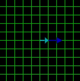
A cyan basis vector and a blue vector. The separation distance for the green lines of the graph paper is 1 cm.

Now imagine that someone wants to use graph paper with spacing of inches. Removing the graph paper we have now and replacing it with the new graph paper will make the unit vector grow by a factor of 2.54.

(new unit vector) = 2.54 * (old unit vector)

We typically work in 3 dimensions at this level. Assume we choose the variables x,y,z for a three dimensional vector:

$x*e^1 + y*e^2 + z*e^3$

A vector can be expressed by the following matrix multiplication:

$x = \begin{bmatrix} e_1 & e_2 & e_3 & ... & e_n \end{bmatrix} \begin{bmatrix} x^1 \\ x^2 \\ x^3 \\ ... \\ x^n \end{bmatrix}$

For the next few examples, we will restrict the examples to three dimensions; this paper believes you can generalize these to n-dimensions.

Below, the matrix with elements S can be used calculate a new basis set from an old basis set.

$\begin{bmatrix} \tilde e_1 & \tilde e_2 & \tilde e_3 \end{bmatrix} = \begin{bmatrix} e_1 & e_2 & e_3 \end{bmatrix} \begin{bmatrix} S_1^1 & S_2^1 & S_3^1 \\ S_2^2 & S_2^2 & S_3^2 \\ S_1^3 & S_2^3 & S_3^3 \end{bmatrix}$

Below, for a matrix like S or T, the superscripts refer to rows and subscripts refer to columns.

$\displaystyle x = \sum_{i=1}^{n} e_ix^i$

$\displaystyle \tilde e_i = \sum_{j=1}^{n} e_j S_i^j$

$\displaystyle e_i = \sum_{j=1}^{n} \tilde e_j T_i^j$

$\displaystyle \tilde x^i = \sum_{j=1}^{n} T_j^i x_j$

The above four equations can be written in what is called Einstein Notation or Implicit Summation Notation:

$x = e_jx^j$
$\tilde e_i = e_jS_i^j$
$e_i = \tilde e_j T_i^j$
$\tilde x^i = T_j^ix^j$
$x^i = S_j^i \tilde x^j$

Use of the Kronecker Delta as a Coordinate Selector:

$\delta_j^i x^j = x^i$

Let V be a vector space with the basis set ${e_1, e_2, e_3, ..., e_n}$ .

To vector space V there corresponds a Dual Vector Space V* with the basis set ${f^1, f^2, f^3, ..., f^n}$ .

Note: we can also say that V is the dual vector space of V* (it works both ways).

We find Vectors in V and we find Dual Vectors (also known as Covectors) in V*. Keep in mind, whether you are a vector or a covector depends on which space got the designation of “V”.